A Distributed Spatial-temporal Data Model and Online Analyst System for Marine Environmental Research
—The GSC Best Practice Data Computing Environment 2018
Zhang, F.1* Bai, Y.2
1. School of Earth Sciences, Zhejiang University, Hangzhou 311300, China;
2. Second Institute of Oceanography, State Oceanic Administration, Qingdao 266000, China
Abstract: A distributed spatial-temporal data model and online analyst system for marine environmental research was recognized by the Geographical Society of China (GSC) as the GSC Best Practice Data Computing Environment 2018. The system is a practical tool for calculating the carbon cycle of marginal seas. To support the massive amount of data generated by satellite remote sensing, on-site vessels, and buoy and shore based stations, a cloud-based, distributed, scalable storage model of carbon flux monitoring data was designed. The key problems of high-scalable storage, high-efficiency retrieval and computing of large-scale marine environmental data were accessed, and we constructed a PB (petabyte)-level, remote sensing carbon flux monitoring data management cloud-based service platform. A heterogeneous, hybrid cloud computing environment was established, and an autonomously controllable, three-dimensional carbon flux remote sensing information service system was developed. The “Ocean Cloud Computing Data Center + Big Data Service Cloud Platform” technology architecture, with independent intellectual property rights, provides a new solution for the on-demand calculation of ocean spatial-temporal big data and diversified service for the Internet of Things in the future.
Keywords: marine carbon sequestration; marine carbon sequestration; big data service; distributed spatial-temporal data model
1 Background
1.1 Scientific Direction and Goals
The ocean absorbs nearly one-third of the CO2 emitted by humans and receives a large amount of terrestrial carbon (about 40% of the anthropogenic CO2). On a long timescale, such as millennial, CO2 can only be removed from the atmosphere by burial in deep-sea marine sediments or forming inert dissolved organic carbon. Therefore, the ocean is the ultimate reservoir of CO2 and is an extremely important component of the Earth’s carbon cycle and global climate change. Marine carbon sequestration (blue carbon sinks) has received wide attention from the international communities, due to issues such as international climate negotiations and carbon trading programs. Satellite remote sensing, which provides long-term observations at high spatial and temporal resolution, is an important tool for calculating the carbon cycle of marginal seas[1].
The goals of this work were to 1) break the bottleneck of high-performance storage and computing technology for marine spatial-temporal data; 2) support the analysis and evaluation of long-timescale, high-precision, high-frequency, large-coverage sea-air and terrestrial- sea carbon flux monitoring data; 3) construct a visualization model of multi-dimensional carbon flux processes to clarify the pattern and variability of major carbon stocks and fluxes; and 4) clarify the processes and mechanisms of dynamic changes in the carbon cycle, including the interaction of natural and human factors.
1.2 Project Organizations and Principle Investigators
There are two organizations jointed the project: (1) Professor Zhang, F. from Zhejiang University, and (2) Professor Bai, Y. from Second Institute of Oceanography (SOA) of China.
2 Data Components
The data structure components of the integrated platform for spatial-temporal distributed storage and computing for marine carbon flux research are listed in Table 1, including dataset name, data parameter type, spatial range and resolution, temporal range and resolution, data sources, etc.
Table 1 The data fabric of the distributed spatial-temporal data model and online analyst system for marine environmental research
|
Dataset name
|
Parameter type
|
Spatial range and resolution
|
Temporal range and
resolution
|
Description
|
|
East India-West Pacific-South China Sea
(EIO-WPO-SCS)
|
Surface suspension concentration
(SSC)
|
(10°N–46°N, 80°E–160°E); 1.8 km
|
May 2010–May 2015; daily average, 10-day average, monthly average, annual average
|
Raw data from NASA, SIO/SOA production
|
|
(10°N–46°N, 80°E–160°E, 1); 5 km
|
2003–2010; 10-day average, monthly average
|
Raw data from NASA, SIO/SOA production
|
|
Chlorophyll concentration (CHL)
|
(10°N–46°N, 80°E–160°E);
1.8 km
|
May 2010–May 2015; daily average, 10-day average, monthly average, annual average
|
Raw data from NASA, SIO/SOA production
|
|
(10°N–46°N, 80°E–160°E); 5 km
|
2003–2010; 10-day average, monthly average
|
Raw data from NASA, SIO/SOA production
|
|
Secchi Disk Depth (SDD)
|
(10°N–46°N, 80°E–160°E);
1.8 km
|
May 2010–May 2015; daily average, 10-day average, monthly average, annual average
|
Raw data from NASA, SIO/SOA production
|
|
(10°N–46°N, 80°E–160°E);
5 km
|
2003–2010; 10-day average, monthly average
|
Raw data from NASA, SIO/SOA production
|
|
Bohai/ Changjiang Estuary (GOB/GOC)
|
Surface suspension concentration (SSC)
|
(27°N–35°N, 119°E–126°E);
500 m
(37°N–41°N, 117°E–123°E); 500 m
|
2011–2017; hourly
|
Raw data from KOSC/GOCI, SIO/SOA production
|
|
Bohai/ Changjiang Estuary (GOB/GOC)
|
Normalized water-leaving radiance at 412 nm (LW1)
|
(27°N–35°N, 119°E–126°E); 500 m
(37°N–41°N, 117°E–123°E); 500 m
|
2011–2017; hourly
|
Raw data from KOSC/GOCI, SIO/SOA production
|
|
Normalized water-leaving radiance at 490 nm (LW3)
|
(27°N–35°N, 119°E–126°E); 500 m
(37°N–41°N, 117°E–123°E); 500 m
|
2011–2017; hourly
|
Raw data from KOSC/GOCI, SIO/SOA production
|
|
Normalized water-leaving radiance at 555 nm (LW4)
|
(27°N–35°N, 119°E–126°E); 500 m
(37°N–41°N, 117°E–123°E); 500 m
|
2011–2017; hourly
|
Raw data from KOSC/GOCI, SIO/SOA production
|
|
Normalized water-leaving radiance at 660 nm (LW5)
|
(27°N–35°N, 119°E–126°E); 500 m
(37°N–41°N, 117°E–123°E); 500 m
|
2011–2017; hourly
|
Raw data from KOSC/GOCI, SIO/SOA production
|
|
Normalized water-leaving radiance at 680 nm (LW6)
|
(27°N–35°N, 119°E–126°E); 500 m
(37°N–41°N, 117°E–123°E); 500 m
|
2011–2017; hourly
|
Raw data from KOSC/GOCI, SIO/SOA production
|
|
Normalized water-leaving radiance at 745 nm (LW7)
|
(27°N–35°N, 119°E–126°E); 500 m
(37°N–41°N, 117°E–123°E); 500 m
|
2011–2017; hourly
|
Raw data from KOSC/GOCI, SIO/SOA production
|
|
Normalized water-leaving radiance at 865 nm (LW8)
|
(27°N–35°N, 119°E–126°E); 500m
(37°N–41°N, 117°E–123°E); 500 m
|
2011–2017; hourly
|
Raw data from KOSC/GOCI, SIO/SOA production
|
|
Global waters (GLOBAL)
|
Chlorophyll concentration (CHL)
|
(90°S–90°N, 180°W–180°E); 4 km
|
1997–2016; daily average,
monthly average
|
From ESA standard products, multi- satellite fusion products
|
|
(90°S–90°N, 180°W–180°E); 4 km
|
Jul. 2002 to publication date; daily
average, monthly average
|
From NASA, Aqua/MODIS products
|
|
(90°S–90°N, 180°W–180°E); 9 km
|
Sep. 1997–Dec. 2010; daily
average, monthly average
|
From NASA, SeaWiFS products
|
|
(90°S–90°N, 180°W–180°E); 4 km
|
2002 to publication date; daily average,
monthly average
|
From NASA, VIIRS products
|
|
Sea surface temperature (SST)
|
(90°S–90°N, 180°W–180°E); 25 km
|
1981 to publication date; daily average
|
From NOAA, AVHRR products
|
|
(90°S–90°N, 180°W–180°E); 25 km
|
Jun. 2002 to publication date; daily average
|
From RSS, MW_IR products
|
|
|
Sea surface wind field (SSW)
|
(90°S–90°N, 180°W–180°E); 25 km
|
1987–2017; six hours, monthly average
|
From RSS, CCMP products
|
|
|
|
(90°S–90°N, 180°W–180°E); 25 km
|
Feb. 2003 to publication date; daily average, monthly average
|
From RSS, Windsat products
|
|
Global waters (GLOBAL)
|
Net primary productivity (NPP)
|
(90°S–90°N, 180°W–180°E); 9 km
|
Sep. 1997–Dec. 2010; monthly average
|
From the University of Oregon, SeaWiFS NPP products
|
|
|
(90°S–90°N, 180°W–180°E); 9 km
|
2012 to publication date; monthly average
|
From the University of Oregon, VIIRS NPP products
|
|
Sea surface salinity (SSS)
|
(90°S–90°N, 180°W–180°E); 25 km
|
Sep. 2016 to publication date; monthly average
|
From RSS, SMAP products
|
|
(90°S–90°N, 180°W–180°E); 25 km
|
Jul. 2009 to publication date; monthly average
|
From ESA, SMOS products
|
|
(90°S–90°N, 180°W–180°E); 25 km
|
2011–2015; monthly average
|
From NASA, Aquaris products
|
|
Atmospheric CO2 partial pressure (ACP)
|
(90°S–90°N, 180°W–180°E); 25 km
|
Daily average
|
From NOAA NCEP, model products
|
|
Remote sensing reflectance (Rrs)
|
(90°S–90°N, 180°W–180°E); 4 km
|
Jul. 2002 to publication date; daily average, monthly average
|
From NASA, Aqua/ MODIS products
|
|
(90°S–90°N, 180°W–180°E); 9 km
|
Sep. 1997–Dec. 2010; daily average, monthly average
|
From NASA, SeaWiFS products
|
|
(90°S–90°N, 180°W–180°E); 4 km
|
2012 to publication date; daily average, monthly average
|
From NASA, VIIRS products
|
|
Photosynthetically active radiation (PAR)
|
(90°S–90°N, 180°W–180°E); 4 km
|
Jul. 2002 to publication date; daily average, monthly average
|
From NASA, Aqua/MODIS products
|
|
(90°S–90°N, 180°W–180°E); 9 km
|
Sep. 1997–Dec. 2010; daily average, monthly average
|
From NASA, SeaWiFS products
|
|
(90°S–90°N, 180°W–180°E); 4 km
|
2012 to publication date; daily average, monthly average
|
From NASA, VIIRS products
|
|
Particulate organic carbon (POC)
|
(90°S–90°N, 180°W–180°E); 4 km
|
Jul. 2002 to publication date; daily average, monthly average
|
From NASA, Aqua/ MODIS products
|
|
(90°S–90°N, 180°W–180°E); 9 km
|
Sep. 1997–Dec. 2010; daily average, monthly average
|
From NASA, SeaWiFS products
|
|
(90°S–90°N, 180°W–180°E); 4 km
|
2012 to publication date; daily average, monthly average
|
From NASA, VIIRS products
|
|
Particulate inorganic carbon (PIC)
|
(90°S–90°N, 180°W–180°E); 4 km
|
Jul. 2002 to publication date; daily average, monthly average
|
From NASA, Aqua/ MODIS products
|
|
(90°S–90°N, 180°W–180°E); 9 km
|
Sep. 1997 to Dec. 2010; daily average, monthly average
|
From NASA, SeaWiFS products
|
|
(90°S–90°N, 180°W–180°E); 4 km
|
2012 to publication date; daily average, monthly average
|
From NASA, VIIRS products
|
|
|
Surface suspension concentration (SSC)
|
(90°S–90°N, 180°W–180°E); 4 km
|
Jul. 2002 to publication date; daily average, monthly average
|
Raw data from NASA Aqua/ MODIS, SIO/SOA production
|
|
|
|
(90°S–90°N, 180°W–180°E); 9 km
|
Sep. 1997–Dec. 2010; daily average, monthly average
|
Raw data from NASA/SeaWiFS, SIO/SOA production
|
|
|
|
(90°S–90°N, 180°W–180°E); 4 km
|
2012 to publication date; daily average, monthly average
|
Raw data from NASA/VIIRS, SIO/SOA production
|
|
Global waters (GLOBAL)
|
Colored dissolved organic matter absorption coefficient at 443 nm (ACD)
|
(90°S–90°N, 180°W–180°E); 4 km
|
Jul. 2002 to publication date; daily average, monthly average
|
Raw data from NASA Aqua/ MODIS, SIO/SOA production
|
|
(90°S–90°N, 180°W–180°E); 9 km
|
Sep. 1997–Dec. 2010; daily average, monthly average
|
Raw data from NASA/SeaWiFS, SIO/SOA production
|
|
(90°S–90°N, 180°W–180°E); 4 km
|
2012 to publication date; daily average, monthly average
|
Raw data from NASA/VIIRS, SIO/SOA production
|
|
Particulate back-scattering coefficient (bbp)
|
(90°S–90°N, 180°W–180°E); 4 km
|
Jul. 2002 to publication date; daily average, monthly average
|
Raw data from NASA Aqua/ MODIS, SIO/SOA production
|
|
(90°S–90°N, 180°W–180°E); 9 km
|
Sep. 1997–Dec. 2010; daily average, monthly average
|
Raw data from NASA/SeaWiFS, SIO/SOA production
|
|
(90°S–90°N, 180°W–180°E); 4 km
|
2012 to publication date; daily average, monthly average
|
Raw data from NASA/VIIRS, SIO/SOA production
|
|
Secchi disk depth (SDD)
|
(90°S–90°N, 180°W–180°E); 4 km
|
Jul. 2002 to publication date; daily average, monthly average
|
Raw data from NASA Aqua/ MODIS, SIO/SOA production
|
|
(90°S–90°N, 180°W–180°E); 9 km
|
Sep. 1997–Dec. 2010; daily average, monthly average
|
Raw data from NASA/SeaWiFS, SIO/SOA production
|
|
(90°S–90°N, 180°W–180°E); 4 km
|
2012 to publication date; daily average, monthly average
|
Raw data from NASA/VIIRS, SIO/SOA production
|
3 Data Computing Environment
The data computing environment includes computer server, model system, software system, network situation, data processing ability, data computing ability, and website dissemination.
3.1 Hardware Environment.
In the existing hardware environment (Table 2), the distributed file system has 200 TB of data storage capability. Hybrid database may support concurrent access of 100 users at the same time. High-performance online processing nodes can provide real-time processing capability of 48 threads at the same time.
3.2 Software System
In order to meet the calculation and service requirements of ocean big data, we used a Hadoop+Spark hybrid processing framework and integrated multi-core and many-core computing technology. We developed a distributed Process-In-Memory architecture, based on Multi-Cloud Coordination, providing unified storage and computing resources for marine distributed databases. This platform provides ocean spatial-temporal big data processing and information mining capabilities, for large-scale ocean carbon flux modeling analysis.
Table 2 The hardware for SatCO2 data sharing platform
|
Number
|
Name
|
Description
|
|
1
|
SatCO2
NameNode
|
Master node of distributed file system
|
|
2
|
SatCO2
DataNode1
|
Subnode of distributed file subsystem
|
|
3
|
SatCO2
DataNode2
|
Subnode of distributed file subsystem
|
|
4
|
SatCO2
Database
|
Hybrid database
|
|
5
|
SatCO2
Webservice1
|
High performance online processing service node
|
|
6
|
SatCO2
Webservice2
|
High performance online processing service node
|
|
7
|
SatCO2
Webservice3
|
High performance online processing service node
|
The main components are as follows (Figure 1):
(1) HDFS: The Hadoop distributed file system (HDFS) is highly fault tolerant and designed to be deployed on low-cost hardware. It provides high throughput to access application data for applications with very large datasets. HDFS relaxes the requirements of POSIX to access data in the file system in the form of streams.
(2) Hadoop Yarn: This splits the JobTracker in MapReduce into two separate services: a global resource manager (ResourceManager) and an ApplicationMaster, unique to each application. The ResourceManager is responsible for the resource management and allocation of the entire system, while the ApplicationMaster is responsible for the management of a single application.
(3) HBase: The Hadoop Database (HBase) is a high-reliability, high-performance, column- oriented, scalable distributed storage system, which is suitable for unstructured data storage databases and is a column-based data storage model.
(4) Hadoop MapReduce: This is Hadoop’s distributed computing framework. Because the framework can easily write applications, these applications can run on large clusters of thousands of commercial machines and process terabytes of data in parallel in a reliable, fault-tolerant manner.
(5) Hive: This is a data warehousing tool based on Hadoop. It can map structured data files into a database table, provide simple SQL query functions, and can convert SQL statements into MapReduce tasks to run.
(6) Oozie: Apache Oozie is a workflow collaboration system. It can configure the workflow to run the ALTER TABLE command, which is responsible for adding a partition containing the last hour of data to Hive. We can also control this workflow to execute every hour. This will ensure that we always see the latest data.
(7) Spark: This is applied to data mining and machine learning and other iterative MapReduce algorithms.
(8) Spark Streaming: This is a real-time computing framework for processing Stream data on Spark, which extends Spark’s ability to handle large-scale Stream data. The basic principle is to divide the Stream data into small time segments (a few seconds) and process the small portion of the data in a batch process.
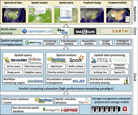
Figure 1 The framework of SatCO2 data sharing platform
(9) MLib: This is Spark’s extensible machine learning library. It provides machine learning algorithms such as classification regression, clustering, association rules, recommendation, dimensionality reduction, optimization, feature extraction screening, statistical methods for feature preprocessing, and algorithm evaluation.
(10) Graphx: A distributed graph computing framework, based on the Spark platform, that provides a simple and easy-to-use interface for graph computing and graph mining. It provides a stack of data solutions based on Spark, which can easily and efficiently complete a set of pipeline operations for graph calculations, greatly facilitating the processing of distributed graph.
3.3 Calculation Ability
(1) Data connection calculation
A new spatial connection algorithm, with embedded index-based concurrent spatial- temporal data retrieval technology and Spark-based in-memory database computing technology, combining the methods of cloning connection and single dataset index external storage space connection, was developed. The new spatial connection algorithm, based on distributed memory computing, was implemented using the Spark parallel programming model. The algorithm first uses a spatial grid to achieve space partitioning. Next, the partitions are connected; the results are analyzed using a re-division model; and the partitions are iteratively re-divided according to the condition. Finally, each partition is processed in parallel using the R*tree single dataset indexing method to obtain the final result of the spatial connection. The results are compared with the spatial connection algorithms proposed by SJMR, SpatialHadoop, Hadoop-GIS, and the SpatialSpark platform. The operation involved 164,448,446 road networks, 72,729,686 plots, 5,857,442 linear water systems, 2,298,808 surface water systems, and 121,960 landmark polygons. Figures 2a and 2b illustrate the performance advantage of our algorithm.
|
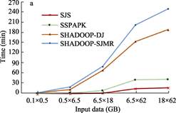
(a) With data volume changes 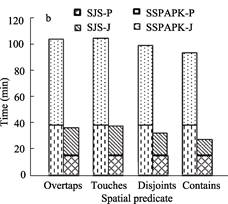
(b) With different spatial predicates
Figure 2 Performance comparison of spatial connections among different algorithms
Figure 3 Relationship of program running time and NUMMU
|
(2) Marine remote sensing image processing test
In a remote sensing image processing performance test, a single task was completed in 20 s and 20,000 tasks took 0.17 hours. With the increase in the number of angle segments, the running speed advantage of the program after parallelization gradually became significant. When the number of angle segments reached 25, the parallelized program ran 64.6 times faster than the stand-alone operation (Figure 3).
(3) Visualization of spatial-temporal processes
We visualized the characteristics of carbon concentration data; designed a progressive data transmission strategy between memory and video memory to cope with the scheduling problem of four-dimensional, large-scale spatial-temporal data; implemented a large-
scale particle state update and half-angle slicing technology based on CUDA; and implemented GPU programming rendering to achieve particle rendering[17].
3.4 Service Website
The public welfare information service system for marine remote sensing is a B/S system version of the Sea-Gas Carbon Dioxide Flux Remote Sensing Monitoring and Evaluation System (SatCO2) (IssCO2 B/S public version). The system provides remote sensing product display and basic quantitative data analysis functions for conventional environmental parameters in the China Sea and adjacent sea areas, and provides the public with a quick query of marine remote sensing information.
Website: http://www.satCO2.com
4 Scientific Achievements
Global climate change caused by the emission of greenhouse gases, such as CO2, seriously threatens human life and economic development. The United Nations has led international negotiations on cutting carbon emissions. China is the largest developing country in the world and one of the highest emitters of CO2. Coordinating energy conservation, emissions reduction, and economic development, to meet international carbon reduction responsibilities, is a huge challenge for China. There is an urgent need to quantify China’s carbon flux and possible carbon sinks. According to the 2013 report of the Global Carbon Project, about 45% of the CO2 emitted by human activities remains in the atmosphere, 27% is absorbed by the oceans, and 28% goes to plants. Therefore, accurate estimation of the marine carbon budget is necessary, in order to understand the global carbon cycle and assess climate change[2]. It is important to construct a long-term, stable ocean CO2 flux monitoring and evaluation system, to obtain reliable sea-gas CO2 flux evaluation results, using remote sensing data.
4.1 A Semi-analytical Remote Sensing Model of Seawater CO2 Partial Pressure
A semi-analytical model of seawater pCO2 (MSAA-pCO2) was developed. The case study area was the portion of the East China Sea affected by Yangtze River freshwater. A salinity remote sensing inversion model of the Yangtze River freshwater surface and a high resolution distribution of the freshwater and its variability over a decade, were obtained for the first time[3]. The project also analyzed the impact of the Yangtze River freshwater on the phytoplankton algal blooms in the offshore area. Included in the model were the thermodynamic, horizontal and vertical mixing, and biological effects. We found that, compared with traditional single- parameter or multi-parameter empirical fit models, the mechanistic-based semi-analytic-
algorithm (MSSA) model is a better solution for the problem of pCO2 remote sensing inversion in complex offshore water bodies (Figure 4). Since the model is based on physio-biochemical mechanisms, it can be applied to other marginal sea systems affected by large rivers.
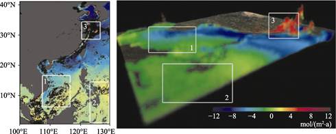
Figure 4 Particle rendering of CO2 spatiotemporal process
4.2 Estimation of Dissolved Organic Carbon Transport Flux Using Satellite Remote Sensing and Numerical Simulation
The project used satellite remote sensing inversion to obtain the surface dissolved organic carbon (DOC) concentration in the East China Sea. The DOC profile distribution model was used to estimate the three-dimensional distribution of DOC concentration[4]. The three-dimensional flow field in the East China Sea was calculated with numerical simulation. Using the remote sensing DOC and simulated flow fields, we estimated the DOC horizontal transport flux in the East China Sea. The results showed that in the Yangtze River estuary, along the coast of Fujian and Zhejiang provinces, the Taiwan Strait, and the Kuroshio region, the DOC flux was high throughout the year, but there were seasonal changes. In the East China Sea shelf, there were three DOC transport belts, from west to east. The transport belt was strong in the summer half-year (from April to September) and weak, sometimes even absent, in the winter half-year (from October to March). In addition, there was a DOC transport belt that extended from the Taiwan Strait to the north and reached the Yangtze River estuary. The largest annual average DOC flux net input was from the Taiwan Strait into the East China Sea, reaching 30.65 Tg C/a, primarily from the eastern side of the Taiwan Strait. The second strongest is the Kuroshio DOC input, which is 18.75 Tg C/a at the 200 m isobath, which comes primarily from the slope in 26°N-26.5°N. The DOC net output of the East China Sea is mainly located at the northern boundary (32°N), reaching -52.75 Tg C/a, primarily from the 100-200 m outer shelf.
4.3 Development of a First Generation Sea-air CO2 Flux Data Product Covering China’s Adjacent Waters (2000-2014)
The method described in the previous section was used to determine the monthly mean sea-level CO2 remote sensing products in China’s adjacent waters (2000-2014). These included atmospheric CO2 partial pressure, seawater CO2 partial pressure, sea-gas CO2 partial pressure difference, and sea-gas CO2, with 1 km resolution. Large-scale navigation data for 15 voyages covering all seasons in China’s Yellow Sea, East China Sea, and South China Sea were obtained. This data proved that, in complex water bodies with high dynamic changes (200-900 μatm) in the offshore area, the average deviation of CO2 partial pressure in remote sensing inversion was less than 35 μatm, the average deviation of atmospheric CO2 partial pressure was less than 10 μatm, and the average deviation of sea-gas CO2 flux was less than ±4.2 mmol C/(m2 day)[9–10].
4.4 Examination of Ecological Changes in the Marginal Seas of the Eurasian Continent, (2003-2014)
Ecosystems changes of 12 marginal seas in the Eurasian continent (2003-2014) were found using the system[5–7]. The results show that the temperature of all marginal seas increased, with a greater increase in the closed marginal seas, including the Black Sea, Baltic Sea, Sea of Japan, Mediterranean Sea, and Persian Gulf. Photosynthetically active radiation generally decreased, but it was not significant for the European marginal seas. Similar to sea surface temperature changes, seawater transparency increased in all marginal seas, with the largest increase rate of 3.02%/a occurring in the Persian Gulf (0.25 m/a, P = 0.0003)[6]. The relationship between sea surface temperature and chlorophyll concentration indicates the complexity of the effects of global warming on phytoplankton[15–16].
4.5 Scientific Findings in the East China Sea
The system was used to estimate the three-dimensional distribution of DOC concentration in the East China Sea[11–12]. The results demonstrated that along the coast of Fujian and Zhejiang provinces, in the Yangtze River estuary, in the Taiwan Strait, and in the Kuroshio region, DOC flux was high throughout the year, but there were seasonal changes[8]. On the East China Sea shelf, there were three DOC transport zones from west to east, which was strong in the summer half-year and weak, or even absent, in the winter half-year. In addition, there was a DOC transport zone that extended from the Taiwan Strait to the north and reached the Yangtze River estuary. The annual average DOC flux from the Taiwan Strait to the East China Sea was the largest. The DOC output in the East China Sea was located mainly at the northern boundary (32°N), primarily output from the 100-200 m outer shelf[1].
5 Conclusion
The project team developed a remote sensing assessment information service system, for ocean carbon flux (SatCO2). More than 130 researchers from 15 countries jointed the application training program in 2016. The data computing environment may be applied further for technical supporting for integrated application of marine environmental monitoring data, for assisting energy conservation and emission reduction decision-making; and for developing new data products and discoveries.
References
[1] Bai, Y., Cai, W. J., He, X., et al. A mechanistic semi-analytical method for remotely sensing sea surface pCO2 in river-dominated coastal oceans: a case study from the East China Sea [J]. Journal of Geophysical Research: Oceans, 2015, 120(3): 2331–2349. DOI: 10.1002/2014JC010632.
[2] Li, T., Pan, D., Bai, Y., et al. Satellite remote sensing of ultraviolet irradiance at the ocean surface [J]. Acta Oceanologica Sinica, 2015, 34(6): 101–112. DOI: 10.1007/s13131-015-0690-z.
Li, T., Bai, Y., Li, G., et al. Effects of ultraviolet radiation on marine primary production with reference to satellite remote sensing [J]. Frontiers of Earth Science, 2015, 9(2): 237–247. DOI: 10.1007/s11707 -014-0477-0.
[3] Liu, D., Pan, D., Bai, Y., et al. Remote sensing observation of particulate organic carbon in the Pearl River estuary [J]. Remote Sensing, 2015, 7(7): 8683–8704. DOI:10.3390/rs70708683
[4] He, X. Q., Pan, D. L., Yan, B., et al. Recent changes of global ocean transparency observed by SeaWiFS [J]. Continental Shelf Research, 2016, 143: 159–166. http://dx.doi.org/10.1016/j.csr.2016.09.011, 2016.
[5] Hu, Z. F., Pan, D. L., He, X. Q., et al. Assessment of the MCC method to estimate sea surface currents in highly turbid coastal waters from GOCI [J]. International Journal of Remote Sensing, 2017, 38(2): 572–597. DOI: 10.1080/01431161.2016.1268737.
[6] Hu, Z. F., Pan, D. L., He, X. Q., et al. Diurnal variability of turbidity fronts observed by geostationary satellite ocean color remote sensing [J]. Remote Sensing, 2016, 8: 147. DOI: 10.3390/rs8020147.
[7] Hu, Z. F., Wang, D. P., Pan, D. L., et al. Mapping surface tidal currents and Changjiang plume in the East China Sea from Geostationary Ocean Color Imager [J]. Journal of Geophysical Research, 2016, 121: 1–10. DOI: 10.1002/2015JC011469.
[8] Song, X. L., Bai, Y., Cai, W. J., et al. Remote sensing of sea surface pCO2 in the Bering Sea in summer based on a mechanistic semi-analytical algorithm (MeSAA) [J]. Remote Sensing, 2016, 8(7): 558. DOI: 10.3390/rs8070558.
[9] Song, X., Bai, Y., Hao, Z., et al. Controlling factors analysis of pCO2 distribution in the Western Arctic Ocean in summertime [J]. Proceedings of SPIE, 2015, 9638: 96380U. DOI: 10.1117/12.2194668.
[10] Wang, H. J., Dai, M. H., Liu, J. W., et al. Eutrophication-Driven Hypoxia in the East China Sea off the Changjiang estuary [J]. Environmental Science & Technology, 2016, 50(5): 2255–2263.
[11] Qian, W., Dai, M. H., Xu, M., et al. Non-local drivers of the summer hypoxia in the East China Sea off the Changjiang estuary [J]. Estuarine Coastal Shelf Science, 2016, 198(Part B): 393-399. https://dx.doi.org/ 10.1016/j.ecss.2016.08.032.
[12] Zhai, W. D., Zang, K. P., Huo, C., et al. Occurrence of aragonite corrosive water in the North Yellow Sea, near the Yalu River estuary, during a summer flood [J]. Estuarine, Coastal and Shelf Science, 2015, 166(part B): 199–208.
[13] Zhai, W. D., Zhao, H. D. Quantifying air-sea re-equilibration-implied ocean surface CO2 accumulation against recent atmospheric CO2 rise [J]. Journal of Oceanography, 2016, 72(4): 651–659. DOI: 10.1007/s10872-016-0350-8.
[14] Qin, M., Li, Z., Du, Z. Red tide time series forecasting by combining ARIMA and deep belief network [J]. Knowledge-Based Systems, 2017, 125: 39–52. https://doi.org/10.1016/j.knosys.2017.03.027.
[15] Zhang, F., Wang, Y., Cao, M., et al. Deep-learning-based approach for prediction of algal blooms [J]. Sustainability, 2016, 8(10): 1060.
[16] Du, Z. H., Fang, L., Bai Y., et al. Spatio-temporal visualization of air-sea CO2 flux and carbon budget using volume rendering [J]. Computers & Geosciences, 2015, 77: 77–86. DOI: 10.1016/j.cageo.2015.01.004.